All predictions, in particular into the future, are risky for those believing them. But let’s take some risk.

By regression analysis I have identified an empirical formula expressing Temperature anomaly a as a function of CO₂ concentration (as a proxy for all GHG and natural or artificial GHG-like effects), Atlantic Multidecadal Oscillation, and Solar spots. To apply the formula over a certain future time frame, scenarios are needed that describe the possible evolution of the underlying parameters.

Perpetuation of solar spot counts was taken from a regression formulas (see Spots in the observation section), and two coarse simulations were obtained for AMO.

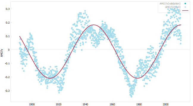
AMO, regression over time

For CO₂, the usual culprit, two scenarios were chosen, with CO₂ as a proxy for all GHG-like forcings:

• Scenario A: CO₂ emissions continue to grow at the same rate as over the past 10 years, this implies a compounded annual growth rate (CAGR) of the CO₂ concentration of 0.67% p.a.
• Scenario B: CO₂ emission growth 50% faster than the current rate, the CAGR of CO₂ concentration is 1.0 %.

These are decisively optimistic scenarios that take into account the potential growth of the old and new economies of the World, without reduction or substitution of fossil fuels by other energy vectors.

Following extrapolations can be seen for scenario A and B:

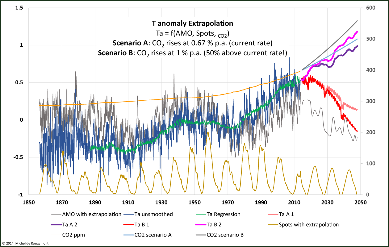
Possible evolution of T anomalies according to empirical formula 1 and 2 and to scenario A and B

And risking a further extrapolation to 2100, the most dramatic scenario B would have burned all proven reserves of fossil fuels, and may push the temperature up by an additional 1.4 °C (2.4 °C since BIE).

In the following chart the empirical formula 1 was abandoned for its lack of physical plausibility beyond the observation period. Two additional CO₂ control scenarios were evaluated,

• Scenario C: freeze at once CO₂ emissions at their current level (10 PgC per year).
• Scenario K: immediately bring back all CO₂ emissions at 8% below their 1991 level and keep them constant. A Kyoto-like scenario.

This is also incredibly new

T anomaly up to 2100 as function of the CO₂ concentration used as a proxy..
Regression formula 2 applied to 4 scenarios after having eliminated variations of AMO
and Spots from formulas in Figure 57.
   A: continuation of historic growth: ΔTa since BIE +2.1 °C.
   B: 50% accelerated growth: ΔTa reaches +2.4 °C.
   C: CO₂ emissions frozen to current level of 10 Gigaton C per year: ΔTa up to +1.9 °C.
   K: Kyoto like cut of all CO₂ emissions by 8% from their 1991 level. ΔTa up to +1.6 °C.
For comparison: current ΔTa is at 0.6 °C (2013)

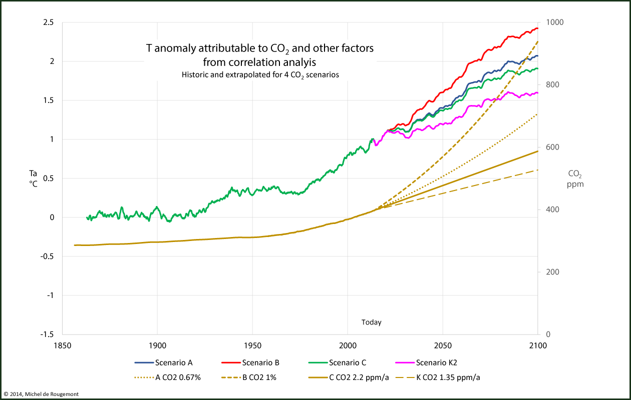
With the restrictive scenario K the additional warming until the end of the century may be 0.6 °C, a difference of 0.8 °C with the high growth scenario B, and 0.5 °C with scenario A (for GHGs and CO₂ only this difference will be smaller after calculating feedbacks, see Action and Feedback)

Reality may lie within the boundaries set by these two impossible scenarios.

Let’s repeat: correlation is not causation, in particular when other parameters play an unquantified role. But what else can be obtained when only three data series are available for analysis over the past 160 years?

Few more or less certain things are also revealed:

• Undoubtedly the emissions proceeding from burning fossil fuels and producing cement impact on the atmospheric CO₂ concentration which, at its turn and by the way of the forcing mechanism, contributes to increasing the global surface temperature. However, this steadily growing CO₂ concentration curve may also be a proxy for other factors such as aerosols, changes of the surface albedo by land use or by soot deposits on ice surface, or yet unidentified natural (continuing exit from the Little Ice Age) or human causes.
• If no naturally occurring steadily ramping factor can be identified, there would be a strong circumstantial evidence that the forcing of approx. 1 °C since the BIE, shown in Figure 59, could be attributed to human industry.
• The impact of oceanic decadal and multi-decadal oscillations and of cyclic solar spots counts have no steady impact on an underlying warming or cooling. As short term disturbances they belong rather to meteorology than to climatology. Other terms with longer cycles, as for example Milankovitch or cosmic rays, may have played a role, but no data is available for the calculated time period.
• In all evaluated regressions, the temperature sensitivity diminishes as CO₂ concentration increases, a logical consequence from the Lambert-Beer law.
• The future temperature remains undefined. We can’t make a valid forecast with these regression formula. However, no spectacular jump of warming or cooling due to CO₂ can be expected with such smooth phenomena, at least none was observed over the past 160 years (see Figure 63). Orders of magnitude have been obtained with which the most dramatic scenario does not lead to any sudden and catastrophic global warming or cooling.
• Scenario comparison: it looks like – with regression formula 2, and using CO₂ as the representative culprit of all warming, a worst case situation – that implementing immediately a Kyoto-like scenario of a global 8% emission cut from their 1991 level would restrict the temperature increase by 0.5 °C as compared with the continuing of the current growth rate, or by 0.8 °C if the rate of growth of emissions would be 50% higher than today. Half a degree in one century is no spectacular contribution to the stopping of climate change.