Correlations & Models

Forcings due to GHGs can be calculated from their concentrations with the formula proposed by Myrhe:

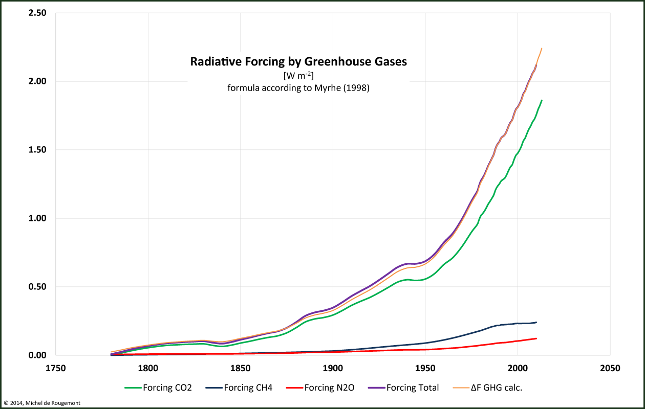
Radiative forcing calculated with Myhre’s formulas based on absorption
of long wave (IR) radiation.

Extrapolation

All predictions, in particular into the future, are risky for those believing them. But let’s take some risk.

By regression analysis, formulas were obtained (link) expressing Temperature anomaly as a function of CO2 concentration (used as a proxy for natural or artificial forcing effects), Atlantic Multidecadal Oscillation, solar spots, and sea level. To apply the formula over a certain future time frame, scenarios are needed that describe the possible evolution of the underlying parameters.
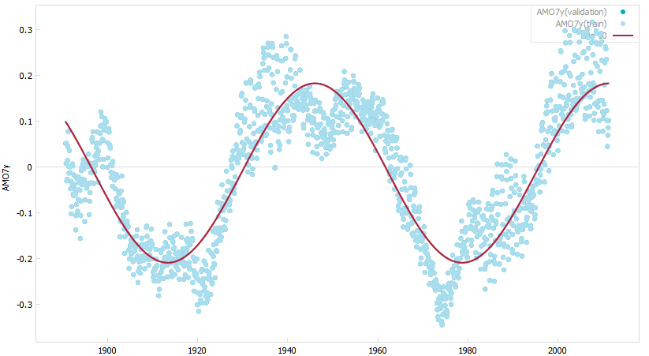
Perpetuation of solar spot counts was taken from a regression formulas (see Solar spot figure), and a simple sinusoidal curve with a period of 65 years was chosen for AMO.

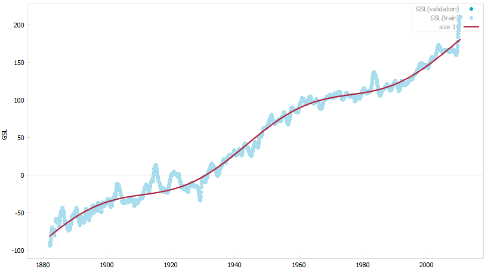
amo regression sea level regression

For the sea level (above on the right), a good fit (R²= 0.986) was obtained with following formula:

GSL = 2.053*Time + 15.073*sin(0.097*Time) - 3950

This formula suggests a steady rise rate of 2 mm per year with fluctuations over a 65 year period.
By the way, the period observed in fluctuations of the rate of rise of the sea level coincides with the period of AMO variations, a parameter based on water temperature at the sea surface. Thermal dilatation may play a role in this.

For CO₂, the usual culprit, four scenarios were chosen, with CO₂ as a proxy for all GHG-like forcings. All scenarios assume that methane and nitrous oxide will continue developing in parallel with the CO₂ rise rate.
A. Do nothing scenario.
The CO₂ concentration continues to grow at the same rate as over the past 10 years, this implies a compounded annual growth rate (CAGR) of 0.67%.
B. Highest carbon scenario until all fossil reserves will have been burned.
An almost unthinkable positive world development scenario.
The CO₂ concentration is as assumed to increase 50% faster than in scenario A. Therefore, the CAGR is 1.0 % p.a.
C. Freeze scenario.
All emissions are maintained at the current level of 9 Pg C per year, no growth. This means that the CO₂ concentration increases steadily by 2.2 ppm every year.
Savings in some countries being cancelled by expansion in others.
K. Kyoto like, lowest carbon scenario.
All emissions are reduced to 8% below the 1991 level, 5.7 Pg C per year.
This was the original aim of the Kyoto protocol. This means that the CO₂ concentration would increase by 1.5 ppm every year.
The control scenarios C and K are supposed to be implemented at once, which is unrealistic (but easy to calculate).
The evolution of the CO₂ concentration will look as follows:

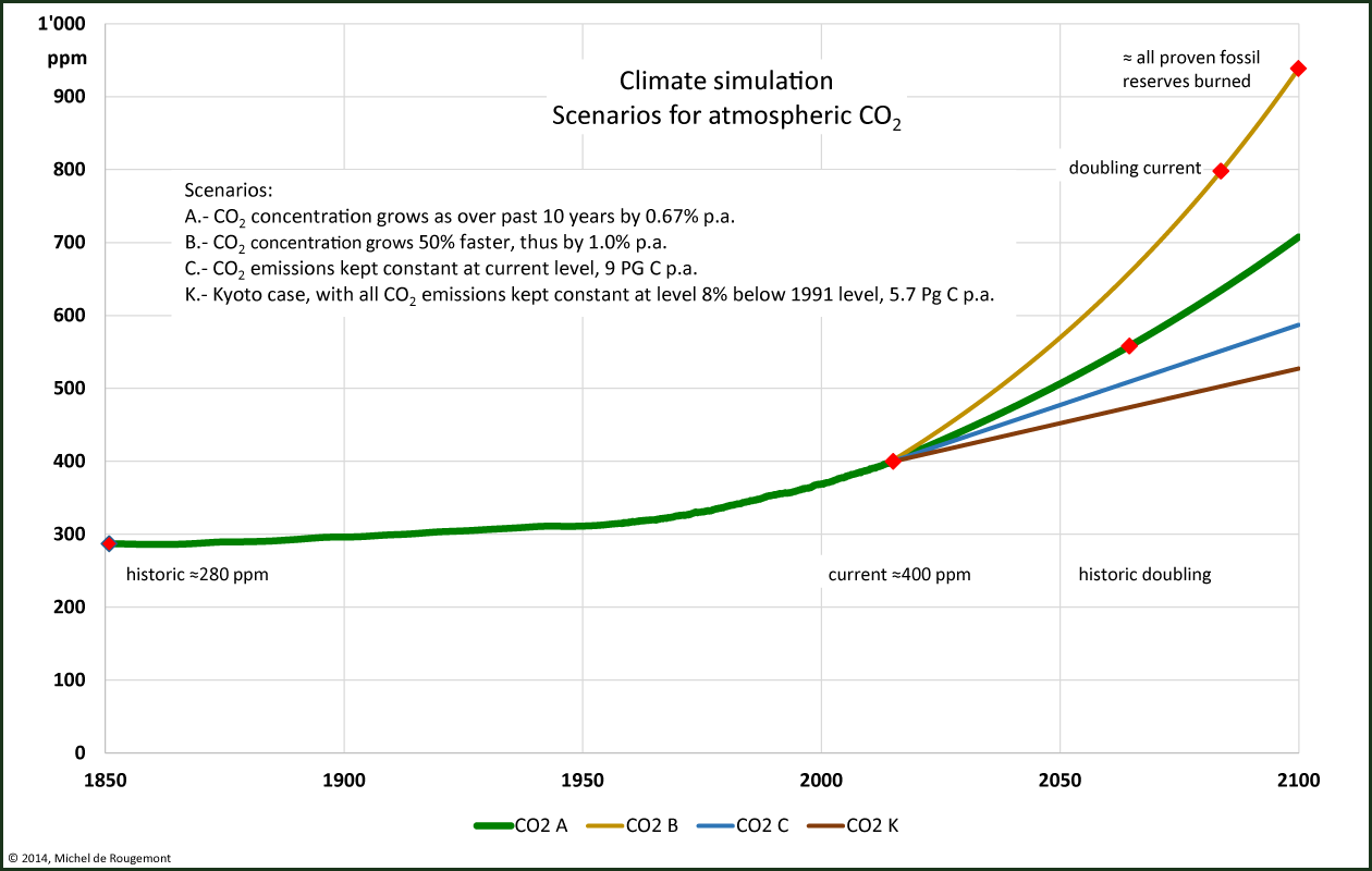
CO₂ Projections of CO₂ concentration according to 4 scenarios

Combining the correlation formulas and the calculation of radiative forcing by CO2 and other GHGs provides the following simulations:

This is an original view, constructed with rigor and

revealing that part of the warming cannot be attributed to CO₂ and other GHGs

Past and future surface temperature evolution.

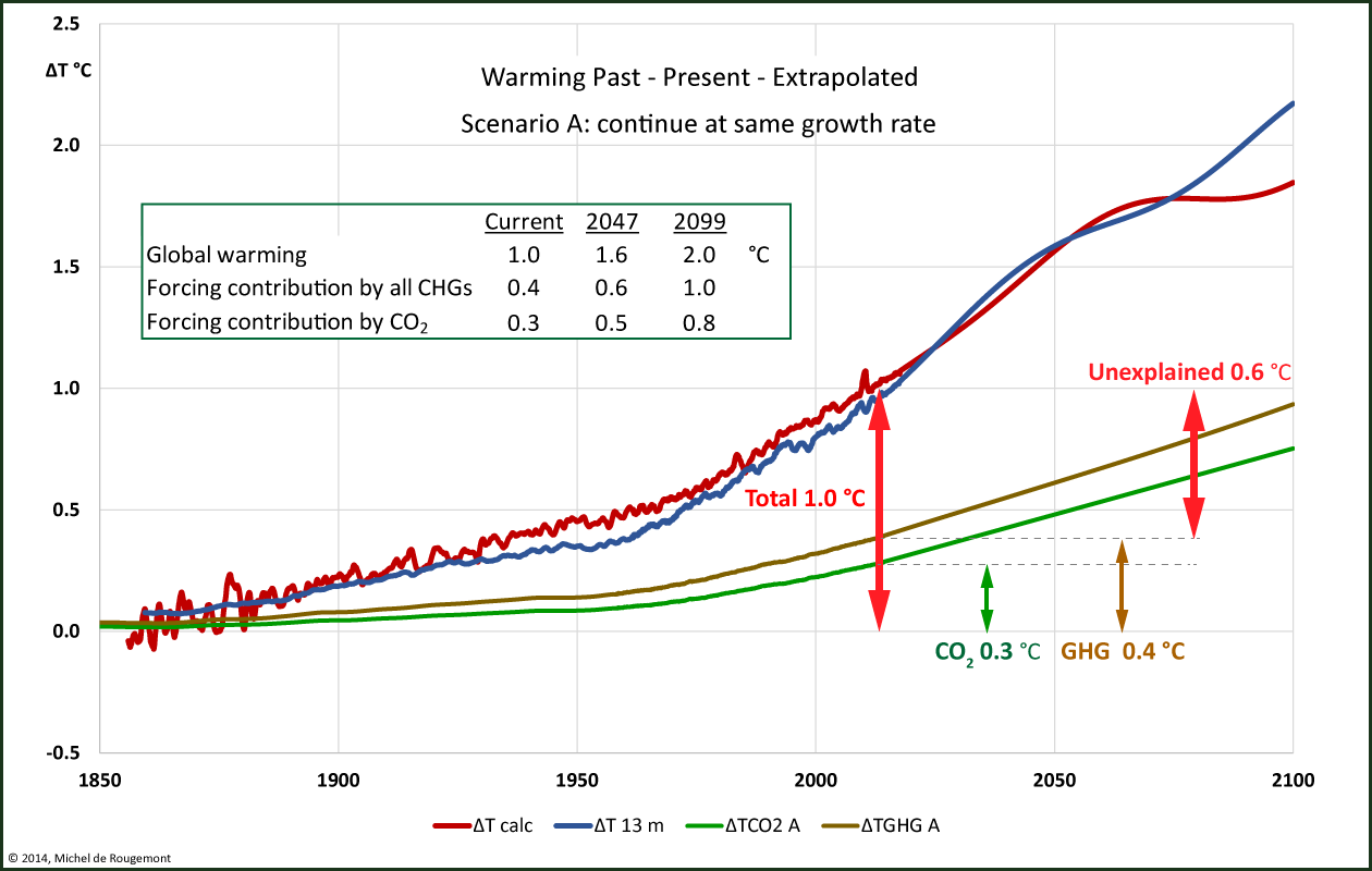
In this chart, the warming as observed and extrapolated is compared with the warming that can be attributed to the known greenhouse gases, taking into account the feedbacks discussed in the past chapter. The calculation for all 4 scenarios can be presented in a table form.

	As of today (2014), compared to pre-industrial era				Additional warming between today and 2047[1]			and in 2099
	ΔT observed overall	ΔT due to all GHGs	ΔT due to CO₂ only	ΔT not explained	ΔT extra-polated overall	ΔT due to all GHGs	ΔT due to CO₂ only	ΔT due to CO₂ only
Scenario A	0.98 °C	0.39 °C	0.28 °C	0.59 °C	0.40	0.21	0.19	0.47
Scenario B					0.59	0.31	0.28	0.70
Scenario C					0.37	0.16	0.14	0.32
Scenario K					0.20	0.11	0.10	0.23

Warming observed, extrapolated from observation, and calculated from radiative forcing according to Myhre’s formulas.
Average feedback factor λ=-1.59 K W^-1m² applied.

Potential effect of carbon dioxide emission reduction.

From the calculations presented here it is possible to show what differences could be achieved in 2047 or at the end of this century according to the chosen scenario.
Some important findings:

Overall, the doing nothing scenario A may result in a temperature increase over the present 2014 situation of 0.4 °C in 2047 and of 1.1 °C in 2099 (1.3 °C and 2.1 °C since BIE).
With this same scenario the contribution of CO₂ alone may be 0.2 °C and 0.5 °C.
The worst case highest carbon scenario for warming – but an ideally best case for economic and social development (scenario B) – may see the temperature increase by 0.6 °C in 2047 and by 1.4 °C in 2099 (1.6 °C and 2.4 °C since BIE).
In this case, the contribution of CO₂ alone would be 0.3 °C and 0.7 °C.
Adopting the best Kyoto-like lowest carbon scenario (K) as compared to doing nothing (A), the warming due to CO₂ would be reduced by 0.1 °C in 2047 and by 0.1 °C in 2099.
In all cases the temperature continues to increase, although more slowly as CHG concentrations increase (logarithmic dependency).

In the above table, “ΔT not explained” is the difference between the observed warming and the one that can be attributed to GHGs only.
To produce the not explained 0.59 °C, an additional primary forcing of 2.91 W m^-2 must be caused by something that has not yet been identified.

In other words, radiative forcing by GHGs cannot explain 60% of the observed warming since the BIE.

To fill the gap, one may be tempted to tune the model, and to apply a large positive feedback factor λ to the whole system, somehow to force the forcing; but this would imply λ = +2.3 K W^-1 m² with which the stability of the climate system would be critically low, which is in full contradiction with Earth’s geological history and with its resilience observed after significant disturbances such as volcanic eruptions or tropical cyclones. And – last but not least – such a high positive feedback would be in full contradiction with all of the published feedback parameters reviewed by IPCC. Therefore, causes other than radiative forcing by GHGs must be found, naturally occurring or man-made[2].

Beginning with the industrial era or continuing the exit from the little ice age, these other factors must show a steady growth pattern up to the present time. Only conjectures can be made, since no other useful observation data is available – if it would be the case, I would have incorporated it in the correlation analysis.

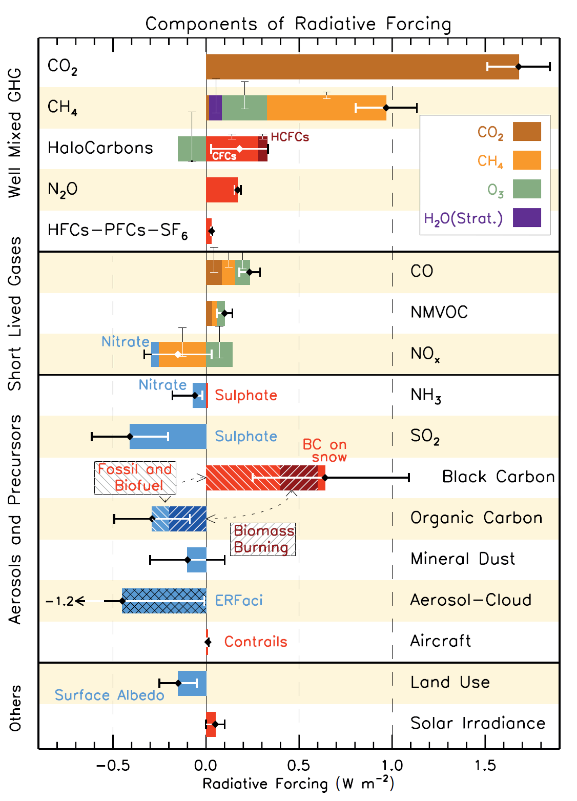
Man-made possible factors with steady growth pattern are:

Increased emissions of fine particles in the form of solid (soot, dust) and liquid (sulphate) aerosols as a result of industry, urbanization, and mobility.
For black carbon, a more recent review of various model calculations made by Bond et al.[3] concludes that “The best estimate of industrial-era climate forcing of black carbon through all forcing mechanisms, including clouds and cryosphere forcing, is +1.1 W m^‑2 with 90% uncertainty bounds of +0.17 to +2.1 W m^-2”. This is much higher than what IPCC has retained in AR5 and would make up for a good part of the gap.
Also it is commented that “The uncertainties in net climate forcing from black-carbon-rich sources are substantial, largely due to lack of knowledge about cloud interactions with both black carbon and co-emitted organic carbon.”
No valid global assessment is currently available on the human contribution to other aerosol formation and of their impact on increased or decreased forcing (low confidence in IPCC’s 5^th report).
Decreased emissions of albedo-contributing dusts and aerosols as consequence of pollution abatement policies.
Change in land use, therefore in surface albedo and emissivity.
Contrails: formation of condensation trails behind high flying airplanes.
Errors in evaluating observation data and in massaging them. This issue is not settled and has been cause for the “climategate” scandal and the hockey stick controversy about wilful manipulation by un ethical scientists.

However, in IPCC’s 5^th report these effects (aside of black carbon) are deemed to be of low magnitude and rather in the cooling than in the warming direction, as summarized in the nearby figure.

Components of radiative forcing for the period 1750 to 2010. From IPCC AR5 WG1 report.

Naturally occurring phenomena with steady growth pattern can be:

Continuing of the exit out of the Little Ice Age, for which no verifiable explanation will ever be available, as also for the entry and exit of Roman Warm Period, Dark Age Cold Period, and Medieval Warm period.
It took approx. 500 years to cool down from RWP to DACP, 400 years to warm up to MWP, and 700 years to cool down again to LIA. The Earth began to get out from the LIA since only 300 years, and we can consider that we are in the midst of this unexplained process.
This situation of “sitting on a growing phase of a longer cycle” could explain a part of the missing gap.

Possible underlying natural phenomena with long periodic pattern, Cause not yet identified.

Phenomena that may be involved are possible changes of the stability of aerosols and thus of cloud formation by varying solar wind (high energy particles) or other cosmic rays.
Indeed, solar impact does not consist only of thermal effects due to electromagnetic radiation in the UV-Vis-IR range. Complex chemical reactions are also induced at altitude as well as at the ground (photosynthesis) that can lead to enhanced or reduced aerosol or cloud formation.
The Cosmics Leaving Outdoor Droplets (CLOUD) experiment at the CERN (cloud.web.cern.ch) studies the influence of cosmic rays on water droplet nucleation to form clouds in presence of aerosols; it is still underway. The link to a potential climate response is far from being quantified.
Regarding clouds and cloud formation, current knowledge is quite scarce. With +0.54 °C per percent cloudiness, the model sensitivity is quite significant. In a previous report, IPCC dared showing how inaccurate observations and models are:

Cloudiness December – February, as observed and evaluated by 11 models
Source: IPCC 2001 assessment report, chapter 8.
Note: the sensitivity of surface temperature to cloudiness is + 0.5 °C for a cloudiness increase by 1 percent.

Other possible interactions with solar activity are shown in the following scheme.

Possible mechanism of solar influence
Source: http://st4a.stelab.nagoya-u.ac.jp/nagoya_workshop_2/pdf/3-2_Miyahara.pdf
This is an area of high awareness but on which little is known about.
Other water feedback, in particular change of phase with large latent energy involved,
Slow release of energy previously accumulated in the oceans.
This would stay in contradiction with the latest IPCC’s assessment that it is virtually certain (IPCC 5^th report) that the upper layer of the oceans has warmed since the BIE, thus not cooled by releasing stored energy.
However, we shall remember that a layer of only 3.4 m has the same heat capacity as the whole atmosphere, and that evaporation involves huge amounts of energy in adiabatic or isothermal conditions. Considering the whole ocean, an accurate time dependent enthalpy balance is yet to be established and validated.

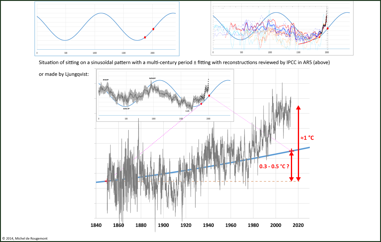
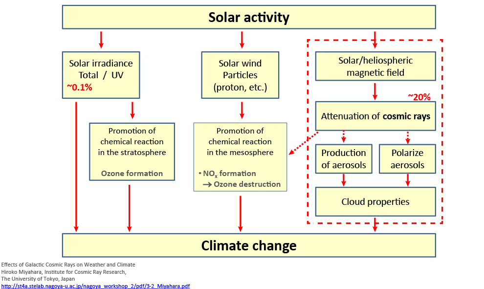
A mix of these phenomena – and others not invented here – may well fill the 2.9 W m^‑2 forcing gap.

In any case, to attribute all ills – if any – to the carbon dioxide molecule appears to be an oversimplification and a considerable exaggeration.

[1] One could be tempted to ask “why 2047 ?“, and the answer being “guess why!”

[2] Women also. The reader is gently asked to consider that in this present text the masculine may, but has not to, mean the feminine, and vice versa. Grammar has no concern for equality, however it is useful to [try to] follow its rules.

[3] Bond, T. C., et al. (2013), Bounding the role of black carbon in the climate system: A scientific assessment, J. Geophys. Res. Atmos., 118, 5380–5552, doi:10.1002/jgrd.50171.